IEO CTD Checker
Use the left side bar to navigate through contents in this page
Introduction
The CTD is a cluster of sensors which measure conductivity (to derive salinity), temperature, and pressure. Other sensors may be added to the cluster, including some that measure chemical or biological parameters, such as dissolved oxygen and chlorophyll fluorescence. The CTD cast collects high resolution data that upon retrieval is downloaded to a computer and specialised software is used to graph and interpret data. However, as stated by the SeaDataNet consortium, many times the collected data are neither easily accessible, nor standardized. They are not always validated and their security and availability have to be insured in the future.
Hundreds of CTD profiles are recorded by Instituto Español de Oceanografía each year and they are routinely incorporated to the SeaDataNet infrastructure network, which in a unique virtual data management system that provide integrated data sets of standardized quality on-line. Sharing data through SeaDataNet is an optimal way of ensuring FAIR principles (Findability, Accessibility, Interoperability, and Reuse).

Thus, each individual record coming from a CTD instrument must be properly flagged to point how confidence is (Quality Flag Scale), data stored in files according to common data transport formats and standard vocabularies and associated metadata created to allow the dataset to be findable and interoperable (Common Data Index).
To achieve this goal, SeaDataNet provides some tools to: i) prepare XML metadata files (MIKADO), ii) convert from any type of ASCII format to the SeaDataNet ODV and Medatlas ASCII formats as well as the SeaDataNet NetCDF format (NEMO) and iii) check the compliance of a file (OCTOPUS). Further analysis and checks can be accomplished with Ocean Data View software among others.
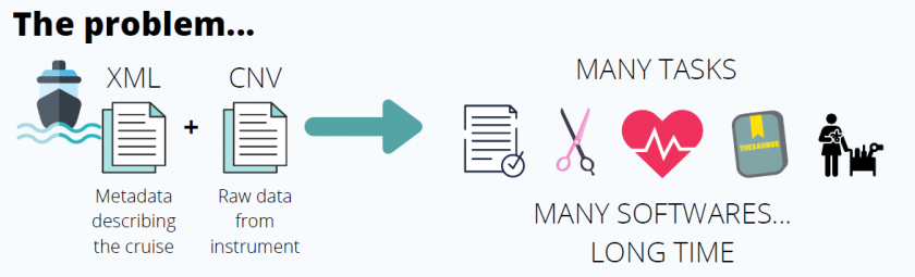
All these tasks are time consuming and require human interaction that can lead to errors or lack of uniformity in data. Taking into account that CTD data usually follows the same format and involves similar processing, a software has been developed to perform all these tasks straightforward. Technically, the software is written in Python and Flask to serve the application through web. To learn about the deployment of this application in a web server, please, read this page.
Even if your goal is not to send the data to SeaDataNet, this application can be useful to detect errors in the stations or share the data with a colleague in a more elegant way.
Prior considerations
The objective of this application is to save time when preparing data and metadata under the SeaDataNet criteria. That is why the vertical profiles of CTD undergo conversions following criteria that adjust to the needs of the Instituto Español de Oceanografía itself. To be noted:
- Only one of the upload or download casts is stored in the resulting file. Downcast is prioritized over upcast whenever possible.
- Records are averaged in 1m bins.
- With exception of the practical salinity, no other derived variables are stored in the resulting file. As they can be easily calculated, this task is left to the end user.
- Redundant sensors are discarded. This limitation comes from the necessary previous existence of the parameter in the P09 vocabulary used in the MedAtlas format. An exception occurs with the temperature variable where up to a maximum of 2 sensors can be processed.
If you need to change some of these criteria, you can download the code, modify it and run it locally on your computer.
How to use the application?
STEP 1 - Uploading
2) Choose between:
-
- simply perform a quality control on the data or
- perform the quality control with output to MedAtllas format and generate metadata.
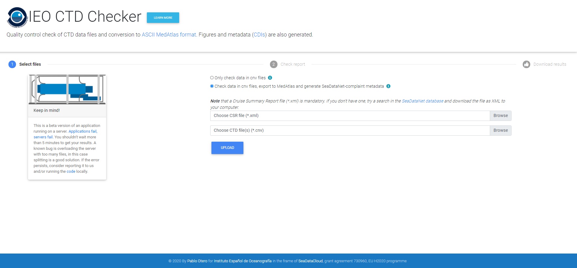
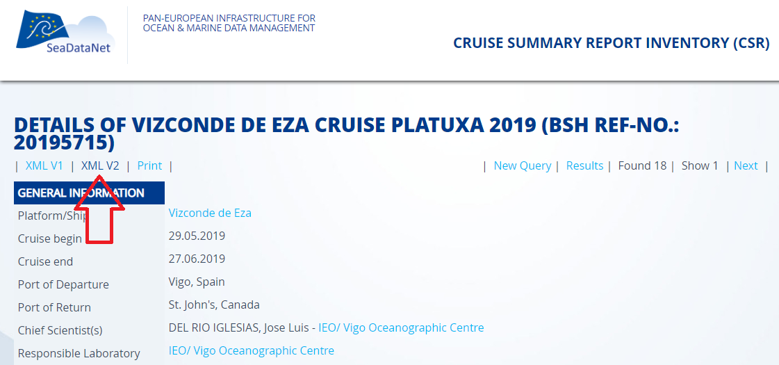
In the first case you only have to provide the cnv files —all at the same time—. In the second case, you must also provide the corresponding Cruise Summary Report (CSR) file. This is a XML file containing information of your research campaign (metadata). Usually, this file is created with MIKADO software at the end of the campaign and submitted to the corresponding National Oceanographic Data Center (NODC). After, the NODC checks and populates this file to the SeaDataNet infrastructure. If you don't have this file, try a search in the SeaDataNet database and download the file as XML V2. For example, if you search the "PLATUXA 2019":
 |
3) Press the "Upload" button and wait for processing. This can take from several seconds to less than 5 minutes. Do not close the browser during processing.
STEP 2 - Reporting
In this step the software parses the files provided and executes various types of tests as a preliminary step to creating the outputs. On the screen, several kind of messages are shown: info (blue), sucess (green), warning (yelllow) and danger/error (red). The user must pay special attention both to warnings (perhaps the software has had to interpret the date or position and its interpretation is not correct) as well as errors. If neccesary, "manually" arrange your files (for example, edit files in your favourite text editor) and repeat again all the process. Here is a screenshot with messages during a processing:
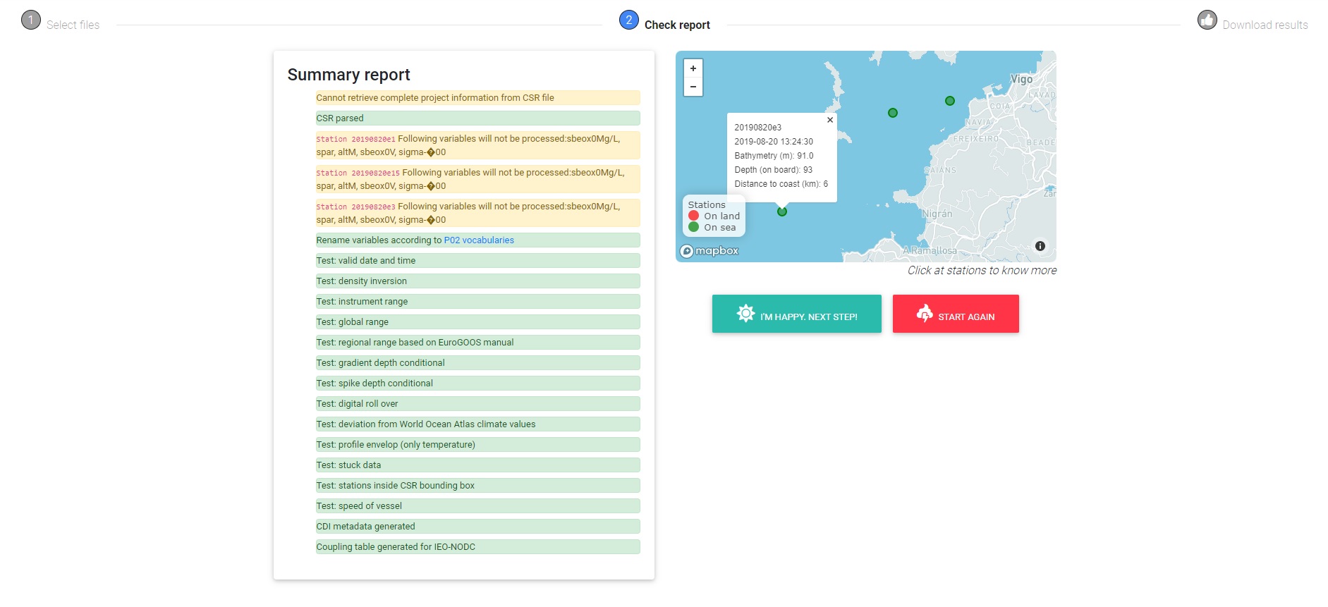 In this case, the CSR file was correctly parsed (green label). Some warnings (yellow) are shown to warn the user that some variables will not be processed.
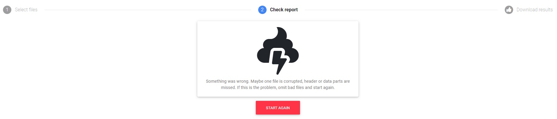
If the software encounters a serious problem of unknown origin, then it displays a message on the screen encouraging a manual review of the files.
STEP 3 - Download and further checks
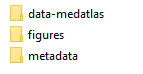
If no errors are detected, a button link to download a zip file appears on the screen. Inside this file we can find: a) a folder "data-cnvFlagged" that includes files following similar scheme that original cnv files, but flagged according to quality checks and created to facilitate its ingestion in NEMO software or a folder "data-medatlas" with all our data in MedAtlas SeaDatanet format, b) some figures with profiles and c) one metadata (CDI) per vertical profile.
If the custodian organization parsed in the CSR file is the Instituto Español de Oceanografía, then an additional file (coupling table) useful to organize the files internally is also generated.
Finally, the responsible technician must validate the data generated. This requires reviewing the generated graphics and, if necessary, carrying out a higher quality control. The use of software such as Ocean Data View allows the result to be directly loaded. On the other hand, Octopus software allows you to check the integrity of the generated medatlas file and convert it to netcdf format. Despite this final supervised review, the app greatly helps save time and catch bugs that might have gone unnoticed.
Why is the existence of a CSR file mandatory?
By so doing, it is ensured that common information is translated unequivocally to formatted data files (MedAtlas format in this case) and also new metadata (CDI). Moreover, after a CSR is submitted to the SeaDataNet infrastructure, a ID is assigned. This ID can therefore be used in the creation of the new CDI files (metadata concerning each CTD cast) properly linking cruise metadata and datasets metadata.
Why MedAtlas format and not netcdf?
It is true that the netcdf format is widely used in oceanography, especially in the field of physical oceanography. However, the MedAtlas format has the advantage of being a text file and has a large amount of information in its header, which makes it largely self-describing. For this reason, it is the format chosen by the IEO as the NODC to share this type of data internationally. In a conversion from MedAtlas to netcdf, some of this information is lost, but the conversion is still possible, something that does not happen from netcdf to MedAtlas.
What can I see on plots?
Salinity and temperature profiles are drawn for each profile whenever. Shaded areas behind profiles indicate climatologic values (mean +/- standard deviation) based on the World Ocean Atlas climatology. An orange or red circle over the profile indicates that a test failed at that point. On the left side a map and a T/S diagram complete the panel.
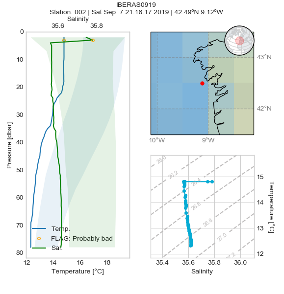
Sometimes it is not possible to adequately interpolate the climatology to the station coordinates —perhaps due to lack of data— so there is a partial or total absence of the shaded area.
Program flow
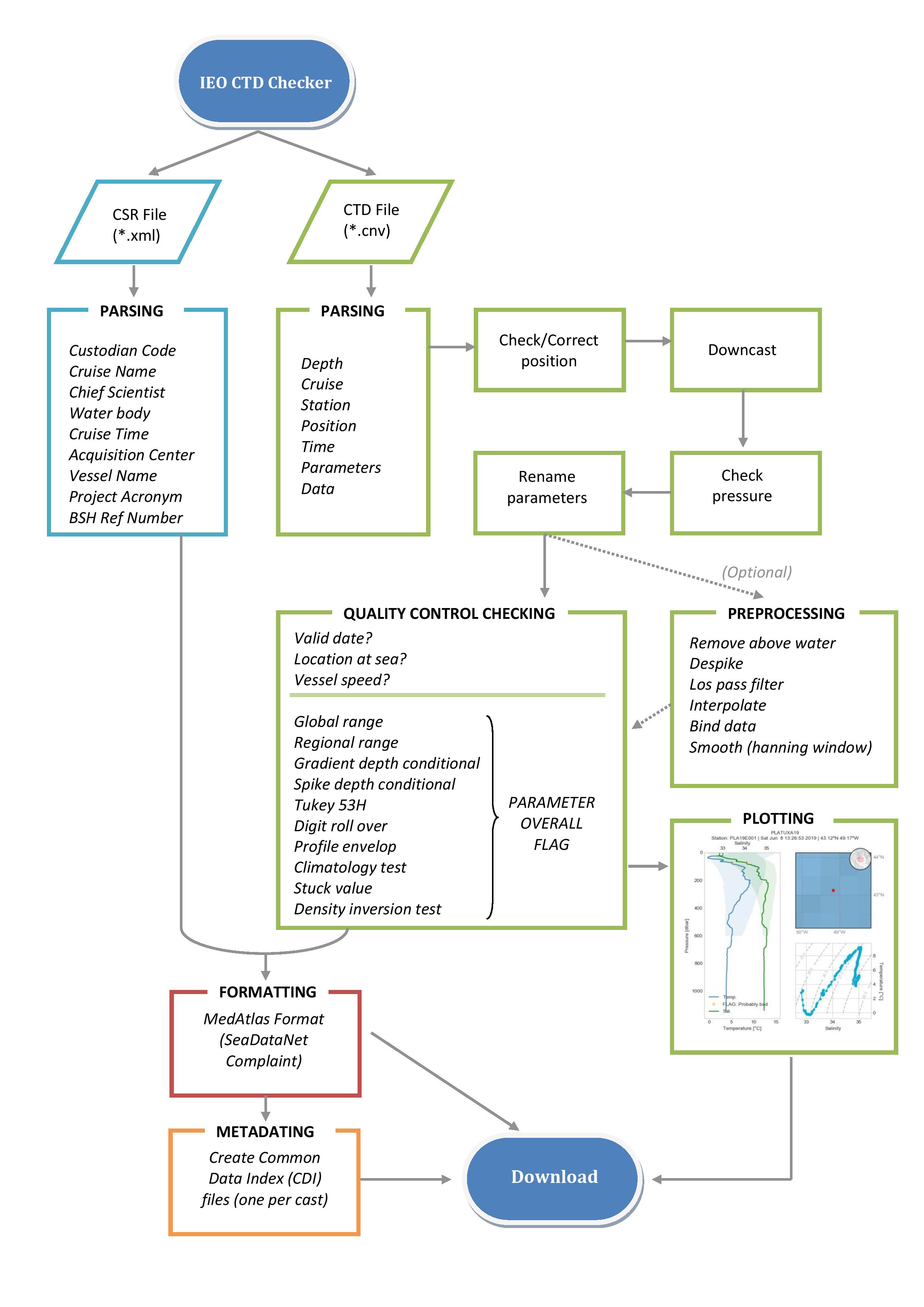
Diagram of the program flow
CSR parsing
When a CSR file is provided, then the file is parsed and some info retained that will help to generate metadata for the CTD vertical profiles (CDI metadata). Like main info from the CSR file will be transferred to CDI files, this means that an important assumption is done: custodian, originator and contact information of the organizations will be the same.
The following table shows a real example of the info extracted from the CSR file after parsing by the application:
| Variable | Value |
| Acquisition Center | IEO, Spanish Oceanographic Institute |
| Chief Scientist | Pablo Carrera |
| Cruise ID | 29VE201603060 |
| Cruise location | ['42.000000', '46.000000', '-11.000000', '1.000000'] |
| Cruise name | CAREVA 0316 |
| Cruise time | 06/03/2016-01/04/2016 |
| Custodian code | 353 |
| Custodian name | IEO, Spanish Oceanographic Institute |
| Originator code | 353 |
| Point of contact code | 353 |
| Project acronym | - |
| Project code | - |
| Project description | - |
| Vessel name | Vizconde de Eza |
| Water body | Northeast Atlantic Ocean (40W) |
In this example, the organization is the same in all cases: custodian, originator and point of contact. The code 353 is the value attributed by the European Directory of Marine Organizations (EDMO). Information about the project was not provided in the CSR file. A good practice is to register all projects in the European Directory of Marine Environmental Research Projects (EDMERP).
The application also extracts some chunks of the CSR xml file that will be directly copied in the CDI file. These chunks are the contact information of the custodian, originator and contact organizations. Below is the code of the custodian organization:
<gmd:CI_Contact>
  <gmd:phone>
    <gmd:CI_Telephone>
      <gmd:voice>
        <gco:CharacterString>+34 91 342 11 00</gco:CharacterString>
      </gmd:voice>
      <gmd:facsimile>
        <gco:CharacterString>+34 91 597 47 70</gco:CharacterString>
      </gmd:facsimile>
    </gmd:CI_Telephone>
  </gmd:phone>
  <gmd:address>
    <gmd:CI_Address>
      <gmd:deliveryPoint>
        <gco:CharacterString>Corazon de Maria, 8</gco:CharacterString>
      </gmd:deliveryPoint>
      <gmd:city>
        <gco:CharacterString>MADRID</gco:CharacterString>
      </gmd:city>
      <gmd:postalCode>
        <gco:CharacterString>28002</gco:CharacterString>
      </gmd:postalCode>
      <gmd:country>
        <sdn:SDN_CountryCode codeList="http://vocab.nerc.ac.uk/isoCodelists/sdnCodelists/cdicsrCodeList.xml#SDN_CountryCode" codeListValue="ES" codeSpace="SeaDataNet">Spain</sdn:SDN_CountryCode>
      </gmd:country>
      <gmd:electronicMailAddress>
        <gco:CharacterString>cedo@ieo.es</gco:CharacterString>
      </gmd:electronicMailAddress>
    </gmd:CI_Address>
  </gmd:address>
  <gmd:onlineResource>
    <gmd:CI_OnlineResource>
      <gmd:linkage>
        <gmd:URL>http://www.ieo.es</gmd:URL>
      </gmd:linkage>
    </gmd:CI_OnlineResource>
  </gmd:onlineResource>
</gmd:CI_Contact>
The info obtained from the CSR file is not shown to the user on the web application. The application is limited to warn if it is not able to parse the file or more than one CSR file is found.
Preprocessing before quality control
The application performs several steps in the backend previous to the quality control phase. All these steps are transparent to the end-user. They are slighty described here:
- Prioritize the selection of the downcast over the upcast.
- Check if profiling CTD Data processing is neccesary. In thas case make it in order according with SeaBird criteria:
- Despike - Wild Edit Seabird-like function with standard deviation 2 and 20 with window size 100
- Low-pass filter: filter a series with time constant of 0.15 s for pressure and sample rate 24 Hz
- Cell thermal mass correction
- Loop edit: remove pressure reversals
- Derive practical salinity if not present
- Bin average to 1m intervals by using interpolation method
- Rename variables according to P09 variables
- Remove duplicate sensors —with the exceptio of the temperature—
- Reorder columns to follow always the same structure. In this way, all your files will be look always similar. Variables will follow the order in the SBE2P09.json (see the "Mapping between variables" section in this document).
Quality Control Flags
“To ensure the data consistency within a single data set and within a collection of data sets and to ensure that the quality and errors of the data are apparent to the user who has sufficient information to assess its suitability for a task.” (IOC/CEC Manual, 1993)
Most of the tests done by the application simply reproduce the procedure recommended by GTSPP. Its real time quality control manual lays out in detail the automatic tests to be carried out on temperature and salinity data (se also SeaDataNet Data Quality Control Procedures manual). In order not to reinvent the wheel, the CoTeDe Python package created by Guilherme P. Castelao has been adapted.
The result of each test for each measurement is coded according to the harmonised scheme of QC Flags used in SeaDataNet:
| Flag | Meaning | Definition |
| 0 | no quality control | No quality control procedures have been applied to the data value. This is the initial status for all data values entering the working archive. |
| 1 | good value | Good quality data value that is not part of any identified malfunction and has been verified as consistent with real phenomena during the quality control process. |
| 2 | probably good value | Data value that is probably consistent with real phenomena but this is unconfirmed or data value forming part of a malfunction that is considered too small to affect the overall quality of the data object of which it is a part. |
| 3 | probably bad value | Data value recognised as unusual during quality control that forms part of a feature that is probably inconsistent with real phenomena. |
| 4 | bad value | An obviously erroneous data value. |
| 5 | changed value | Data value adjusted during quality control. Best practice strongly recommends that the value before the change be preserved in the data or its accompanying metadata. |
| 6 | value below detection |
The level of the measured phenomenon was too small to be quantified by the technique employed to measure it. The accompanying value is the detection limit for the technique or zero if that value is unknown. |
| 7 | value in excess | The level of the measured phenomenon was too large to be quantified by the technique employed to measure it. The accompanying value is the measurement limit for the technique. |
| 8 | interpolated value | This value has been derived by interpolation from other values in the data object |
| 9 | missing value | The data value is missing. Any accompanying value will be a magic number representing absent data. |
The initial status of all data values is 0. If the value exists and all tests are passed, the output flag is set to 1. A fail on the climatology test would return a flag 3, whereas the fail in a more critical test would return 4. If the data value is missing, output flag is set to 9. The overall flag of an individual value will be the highest number obtained from the set of tests.
Quality Control tests
Valid date time
Check if time has a valid format. The time is extracted from the cnv header file according with the following priority:
- NMEA time.
- System Upload Time
- <startTime> tag when CTD is in XML format
- Date and time present in header and typed by technician (based on a search of the keywords "Date" and "Time")
Valid position format
Check if time has a valid format. Prioritize the existence of NMEA positions in the header file. Otherwise, take the position typed by the technician based on keywords like "Latitude", "Latitud", "Longitude" or "Longitud". Verify the format and correct it if discrepancies appear.
Examples of corrections done in the latitude by the application (similar in longitude):
| Original value | Formatted value |
| 43.24971 | 43 14.98N |
| 43.606 | 43 36.36N |
| 43 24820 | 43 14.89N |
| 43 23.18 n | 43 23.18N |
| 43 23,18 n | 43 23.18N |
| -43 23.18S | 43 23.18S |
Modifications in position are always warned to the user. It should have a latitude between -90 and 90, and a longitude between -180 and 180.
Location at sea
Check if the position is at sea, which is evaluated using the distance to coast from the XYLOOKUP Web service. This API relies on OpenStreetMap. If a CTD location is inland then it warns to the user with a message on the screen, It also highlights the position on the map. No quality control flags are assigned at this step beacuse it is expected that the user will be able to detect the error in the file with the warning provided, correct it and process again. If the user is not able to detect the problem, then a global quality control flag 3 should be assigned to the profile.
Many thanks to IOBIS team for sharing this nice API!
Valid depth
As a further step to ensure the validity of the position, it is possible to compare the depth recorded by the echosound (if annotated on the CTD header) and the bathymetry. As in the previous test, bathymetry is obtained from the XYLOOKUP Web service based here on GEBCO and EMODnet Bathymetry data (see references section).
Coherence between CSR metadata ad CTD info
Check if the date and time is in the temporal range indicated in the Cruise Summary Report file.
The test also checks if position is inside the bounding box indicated in the Cruise Summary Report file. There are two possibilities when CTDs are located out the CSR bounding box:
a) The location of one or more CTDs are wrong. To know if a CTD location is wrong, the user can check directly the map shown on the screen in Step 2. To check the depth recorded by the echosound and the depth in the bathymetry can also help to understand if the location is possible. It is frequent that the faults in positions also entail associated a failure in the "vessel speed test"
b) The bounding box reported in the CSR XML file is wrong. In that case you should contact your National Oceanographic Data Center in order to correct the metadata file.
Vessel speed test
Compute speed of the vessel between consecutive stations. A too short navigation time between stations may indicate a problem in geoposition. This test is based in a gross estimation. To the total time elapsed between two stations is subtracted the CTD down and up time of the first station (considering a typical ascent and descent rate of 1m/s). A 10 minutes operation time is also substracted. With the remaining time and the distance between stations, a mean vessel speed is computed and this should not exceed 15 knots. Otherwise, a warning is shown.
Location at Sea
Check if the position is at sea, which is evaluated using a bathymetry with resolution of 1 minute (ETOPO1). It is considered at sea if the interpolated position has a negative vertical level (QC Flag 1). Otherwise, a "probably bad value" is assigned (QC Flag 3).
Pressure increasing test
If there is a region of constant pressure, all but the first of a consecutive set of constant pressures are flagged as bad data. If there is a region where pressure reverses, all of the pressures in the reversed part of the profile are flagged as bad data.
Instrument range
This test checks that records are in the instrument range. The widest range from the various models of SeaBird's CTD has been taken. If a value fails, it is flagged as bad data (QC Flag 4)
Global Range
This test evaluates if the temperature or salinity record is a possible value in the ocean. If not, a QC Flag 4 is assigned. The thresholds used are extreme values, wide enough to accommodate all possible values and do not discard uncommon, but possible, conditions. Examples of current acceptable ranges for temperature and salinity:
- Temperature in range –2.5°C to 40.0°C
- Salinity in range 0 to 41.0 (note that EuroGOOS manual sets 2 as minimum salinity value)
Regional Range
This test applies to temperature and salinity and only to certain regions of the world where conditions can be further qualified. Individual values that fail these ranges are flagged as bad data (QC Flag 4):
- Red Sea
- Temperature in range 21.7°C to 40.0°C
- Salinity in range 2.0 to 41.0
- Mediterranean Sea
- Temperature in range 10.0°C to 40.0°C
- Salinity in range 2.0 to 40.0
- North Western Shelves (from 60N to 50N and 20W to 10E):
- Temperature in range –2.0°C to 24.0°C
- Salinity in range 0.0 to 37.0
- South West Shelves (from 25N to 50N and 30W to 0W):
- Temperature in range –2.0°C to 30.0°C
- Salinity in range 0.0 to 38.0
- Arctic Sea (above 60N):
- Temperature in range –1.92°C to 25.0°C
- Salinity in range 2.0 to 40.0
Gradient (depth conditional)
This test checks the gradient as defined by GTSPP, EuroGOOS and others:

where Vi is the measurement being tested and Vi+1 and Vi-1 the values above and below. This test is failed when the difference between vertically adjacent measurements is too steep (threshold). Note that the test does not consider the differences in depth, but assumes a sampling that adequately reproduces the temperature and salinity changes with depth. Threshold values:
- Temperature: 9.0°C for pressures less than 500 db and 3.0°C for pressures greater than or equal to 500 db.
- Salinity: 1.5 for pressures less 500 db and 0.5 for pressures greater than or equal to 500 db.
Spike (depth conditional)
This test checks if there is a large difference between sequential measurements, where one measurement is quite different from adjacent ones, following:

where Vi is the measurement being tested and Vi+1 and Vi-1 the values above and below. Note that the test does not consider the differences in depth, but assumes a sampling that adequately reproduces the temperature and salinity changes with depth. Threshold values:
- Temperature: 6.0°C for pressures less than 500 db and 2.0°C for pressures greater than or equal to 500 db.
- Salinity: 0.9 for pressures less 500 db and 0.3 for pressures greater than or equal to 500 db.
Spike test Tukey53H
A smooth time series is generated from the median, substracted from the original signal and compared with the standard deviation. This procedure was initially proposed for Acoustic Doppler Velocimeters ("Despiking Acoustic Doppler Velocimeter Data", Derek G. Goring and Vladimir L. Nikora, Journal of Hydraulic Engineering, 128, 1, 2002)
For one individual measurement xi, evaluates as follows:
- V(1) is the median of the five points from Vi-2 to Vi+2
- V(2) is the median of the three points from V(1)i-1 to V(1)i+1
- V(3) is the defined by the Hanning smoothing filter: 1/4(V(2)i-1+2V(2)i+V(2)i+1)
Now, a spike (QC flag 4) is detected if:
|Vi - V(3)|/ > k, where is the standard deviation of the lowpass filtered data (Hamming window of length 12). In this test k is assumed to be 1.5 for both temperature and salinity.
Digit rollover
Only so many bits are allowed to store values in a sensor. This range is not always large enough to accommodate conditions that are encountered in the ocean. When the range is exceeded, stored values roll over to the lower end of the range. This test attempts to detect this rollover (extreme jumps in consecutive measurements):
- Temperature difference between adjacent depths > 10°C
- Salinity difference between adjacent depths > 5
Profile envelop
This test evaluates if temperature is inside different ranges that are depth-dependent. Values have been obtained from Castelao (link to the code):
| Depth (db) | Valid temperature range (ºC) |
| 0-25 | -2 to 37 |
| 25-100 | -2 to 36 |
| 100-150 | -2 to 34 |
| 150-200 | -2 to 33 |
| 200-300 | -2 to 29 |
| 300-1000 | -2 to 27 |
| 1000-3000 | -1.5 to 18 |
| 3000-5500 | -1.5 to 7 |
| >5500 | -1.5 to 4 |
Climatology test
This test compares observed values to climatic values in the region. The bias (observed value minus mean climatologic value) is normalized by the standard deviation obtained from climatology. To pass the test, the absolute value must be below a threshold (set here to 10 for both temperature and salinity). Climatology is obtained from World Ocean Atlas database and extracted afrom any coordinate thanks to Python package oceansdb.
Stuck value
Looks for all measurements in a profile being identical. If this occurs, all of the values of the affected variable are flagged as bad data (QC Flag 4).
Density inversion test
With few exceptions, potential water density σθ will increase with increasing pressure. This test uses values of temperature and salinity at the same pressure level and computes the density (sigma0). The algorithm published in UNESCO Technical Papers in Marine Science #44, 1983 is used. Densities (sigma0) are compared at consecutive levels in a profile. Small inversion, below a threshold that can be region dependant, is allowed (<0.03Kg/m3). If the test fails, both temperature and salinity records are flagged as probably bad (QC Flag 3).
Adjustment of quality control parameters
Some of the quality control tests require threshold values that may vary depending on the variable. In the backend, a file named cfg_IEO.json is the responsible of setting these adjustments in similar way to Castelao (2020). The file is a dictionary composed by the variables to be evaluated as keys, and inside it another dictionary with the tests to perform as keys.
An example of the code found inside cfg_IEO.json:
{"main": {
    "valid_datetime": null,
    "valid_geolocation": null,
    "location_at_sea": {
	    "bad_flag": 3
        },
	"max_speed": 15
    },
"PRES": {
    "instrument_range": {
        "minval": 0,
        "maxval": 10500
        }
    },
"CNDC": {
    "instrument_range": {
        "minval": 0,
        "maxval": 9
        }
    },
"SVEL": {
    "instrument_range": {
        "minval": 1450,
        "maxval": 1600
        }
    },
"DOX1": {
    "instrument_range": {
        "minval": 0,
        "maxval": 40
        }
    },

    [...]

"TEMP": {
    "pstep": null,
    "instrument_range": {
        "minval": -5,
        "maxval": 35
        },
    "woa_normbias": {
        "threshold": 10
        },
    "global_range": {
        "minval": -2.5,
        "maxval": 40
        },
    "regional_range": {
	    "MediterraneanSea": {
			"geometry": {
				"type": "Polygon",
				"coordinates": [
					[
						[30, -6],
						[30, 40],
						[40, 35],
						[42, 20],
						[50, 15],
						[40, 5],
						[30, -6]
					]
				]
			},
			"minval": 10,
			"maxval": 40
           },
	    "RedSea": {
			"geometry": {
				"type": "Polygon",
				"coordinates": [
					[
						[10, 40],
						[20, 50],
						[30, 30],
						[10, 40]
					]
				]
			},
			"minval": 21.7,
			"maxval": 40
           },
	    "North_Western_Shelves": {
			"geometry": {
				"type": "Polygon",
				"coordinates": [
					[
						[50, -20],
						[50, 10],
						[60, 10],
						[60, -20],
						[50, -20]
					]
				]
			},
			"minval": -2.0,
			"maxval": 24
           },
	    "South_West_Shelves": {
			"geometry": {
				"type": "Polygon",
				"coordinates": [
					[
						[25, -30],
						[25, 0],
						[50, 0],
						[50, -30],
						[25, -30]
					]
				]
			},
			"minval": -2.0,
			"maxval": 24
           },
	    "Artic_Sea": {
			"geometry": {
				"type": "Polygon",
				"coordinates": [
					[
						[60, -180],
						[60, 180],
						[90, 180],
						[90, -180],
						[60, -180]
					]
				]
			},
			"minval": -1.92,
			"maxval": 25
           }
        },
    "spike": {
		"threshold": 6.0
        },
    "spike_depthconditional": {
        "pressure_threshold": 500,
        "shallow_max": 6.0,
        "deep_max": 2.0
        },
    "tukey53H_norm": {
        "threshold": 1.5,
        "l": 12
        },
    "gradient": {
	"threshold": 9.0
        },
    "gradient_depthconditional": {
        "pressure_threshold": 500,
        "shallow_max": 9.0,
        "deep_max": 3.0
        },
    "digit_roll_over": 10,
    "rate_of_change": 4,
    "cum_rate_of_change": {
        "memory": 0.8,
        "threshold": 4
    },
    "profile_envelop": [
        ["> 0", "<= 25", -2, 37],
        ["> 25", "<= 100", -2, 36],
        ["> 100", "<= 150", -2, 34],
        ["> 150", "<= 200", -2, 33],
        ["> 200", "<= 300", -2, 29],
        ["> 300", "<= 1000", -2, 27],
        ["> 1000", "<= 3000", -1.5, 18],
        ["> 3000", "<= 5500", -1.5, 7],
        ["> 5500", "<= 12000", -1.5, 4]
        ],
    "anomaly_detection": {
        "threshold": -20.0,
        "features": {
            "gradient": {
                "model": "exponweib",
                "qlimit": 0.013500,
                "param": [1.431385, 0.605537, 0.013500, 0.015567]
                },
            "spike": {
                "model": "exponweib",
                "qlimit": 0.000400,
                "param": [1.078231, 0.512053, 0.000400, 0.002574]
                },
            "tukey53H_norm": {
                "model": "exponweib",
                "qlimit": 0.001614,
                "param": [4.497367, 0.351177, 0.001612, 0.000236]
                },
            "rate_of_change": {
                "model": "exponweib",
                "qlimit": 0.041700,
                "param": [2.668970, 0.469459, 0.041696, 0.017221]
                },
            "woa_normbias": {
                "model": "exponweib",
                "qlimit": 1.615422,
                "param": [0.899871, 0.987157, 1.615428, 0.662358]
                }
            }
        }
    },
Mapping between variables
In the backend, a mapping between SeaBird variables and P09 vocabulary is done. This "new" variable names are used in the MedAtlas formatting. The file SBE2P09.json is where the mapping is set. Here a piece of this file:
{
   "pr":{
      "full_name":"Pressure [db]",
      "name_P09":"PRES"
   },
   "prM":{
      "full_name":"Pressure [db]",
      "name_P09":"PRES"
   },
   "prDM":{
      "full_name":"Pressure, Digiquartz [db]",
      "name_P09":"PRES"
   },
   "prdM":{
      "full_name":"Pressure, Digiquartz [db]",
      "name_P09":"PRES"
   },
   "prSM":{
      "full_name":"Pressure, Strain Gauge [db]",
      "name_P09":"PRES"
   },
   "pr50M":{
      "full_name":"Pressure, SBE 50 [db]",
      "name_P09":"PRES"
   },
   "pr50M1":{
      "full_name":"Pressure, SBE 50, 2 [db]",
      "name_P09":"PRES"
   },
   "t068C":{
      "full_name":"Temperature [IPTS-68, deg C]",
      "name_P09":"TEMP"
   },
   "t4968C":{
      "full_name":"Temperature [IPTS-68, deg C]",
      "name_P09":"TEMP"
   },
   "tnc68C":{
      "full_name":"Temperature [IPTS-68, deg C]",
      "name_P09":"TEMP"
   },
   "tv268C":{
      "full_name":"Temperature [IPTS-68, deg C]",
      "name_P09":"TEMP"
   },
   "t090C":{
      "full_name":"Temperature [IPTS-90, deg C]",
      "name_P09":"TEMP"
   },
 [...]
On the other hand, there is a mapping between P09 variable names and those of the P01 vocabulary, P06 units and IOC codes. The file P09toP01.json contains this mapping:
{
   "PRES":{
      "name_IOC":"SEA PRESSURE sea surface=0",
      "units_IOC":"decibar=10000 pascals",
      "name_P01":"PRESPR01",
      "name_P06":"UPDB",
      "fractional_part": 0
   },
   "TEMP":{
      "name_IOC":"SEA TEMPERATURE",
      "units_IOC":"Celsius degree",
      "name_P01":"TEMPPR01",
      "name_P06":"UPAA",
      "fractional_part": 3
   },
   "TE01":{
      "name_IOC":"SEA TEMPERATURE",
      "units_IOC":"Celsius degree",
      "name_P01":"TEMPPR01",
      "name_P06":"UPAA",
      "fractional_part": 3
   },
   "TE02":{
      "name_IOC":"SEA TEMPERATURE",
      "units_IOC":"Celsius degree",
      "name_P01":"TEMPPR02",
      "name_P06":"UPAA",
      "fractional_part": 3
   },
   "PSAL":{
      "name_IOC":"PRACTICAL SALINITY",
      "units_IOC":"P.S.U.",
      "name_P01":"PSLTZZ01",
      "name_P06":"UUUU",
      "fractional_part": 4
   },
 [...]
Remember to add new variables to these two files, as well as to replicate in the case of secondary sensors
References
- Manual for Real-Time Quality Control of In-situ Temperature and Salinity Data. A Guide to Quality Control and Quality Assurance for In-situ Temperature and Salinity Observations (IOOS, 2014)
- Recommendations for in-situ data Near Real Time Quality Control (EuroGOOS, DATA-MEQ working group, 2010)
- Data Quality Control Procedures (SeaDataNet, 2010)
- Castelao, G. P., (2020). A Framework to Quality Control Oceanographic Data. Journal of Open Source Software, 5(48), 2063, https://doi.org/10.21105/joss.02063
-
The GEBCO_2014 Grid, version 20150318, http://www.gebco.net.
-
EMODnet Bathymetry Consortium (2016): EMODnet Digital Bathymetry (DTM). http://doi.org/10.12770/c7b53704-999d-4721-b1a3-04ec60c87238.